Sun-Synchronous Orbits

Given the Earth's gravitational potential, all the low Earth orbits (LEO) suffer from perturbations in their elements. The right ascension of the ascending node (RAAN) is one of the elements that see a secular perturbation. Hence, we can use this effect to design orbits whose RAAN time derivative matches that of the Earth's orbit around the Sun. In this case, the orbit plane keeps its geometry almost constant regarding the Sun vector. Hence, the apparent local time of the ascending or descending node (LTAN and LTDN) will also be almost invariable, as shown in the following figure:

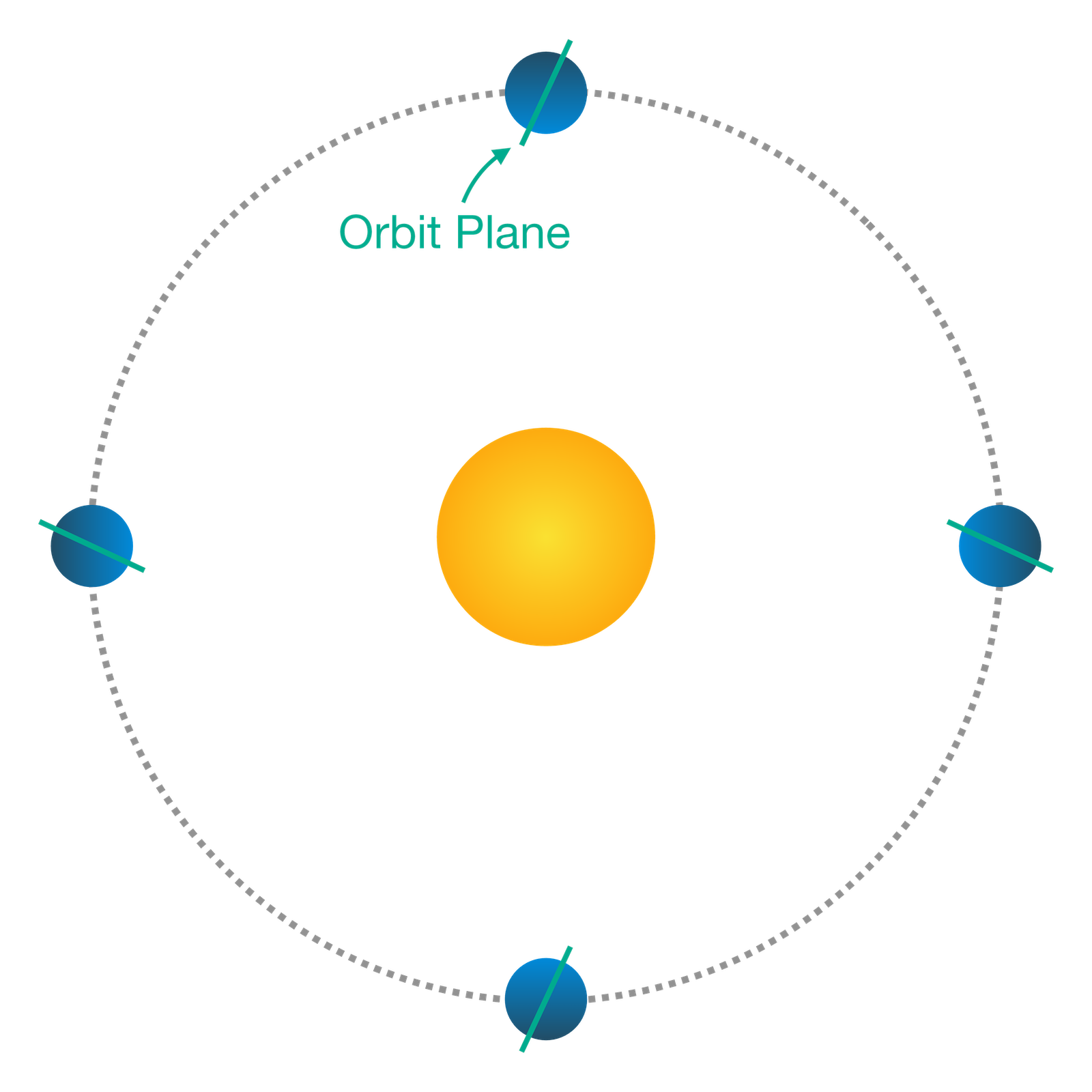
In fact, if the Earth was a perfect sphere, no secular perturbation would be seen in RAAN. Hence, the LTAN would have a variation of 24 hours in a year.

Considering only terms up to $J_2$, which is the dominant effect, the RAAN time derivative is:

\[\frac{d\Omega}{dt} = -\frac{3}{2} J_2 \left(\frac{R_0}{p_0}\right)^2 \bar{n} \cos i_0\ ,\]

where $R_0$ is the Earth's Equatorial radius, $i_0$ is the orbit inclination, $p_0 = a_0 (1 - e_0^2)$, $a_0$ is the orbit semi-major axis, $e_0$ is the orbit eccentricity, and $\bar{n}$ is the perturbed mean-motion, given by:

\[\bar{n} = n_0 \left[1 + \frac{3}{4} J_2 \left(\frac{R_0}{p_0}\right)^2 \sqrt{1 - e_0^2} \left(2 - 3\sin^2 i_0\right)\right]\ ,\]

where $n_0 = \sqrt{\mu / a_0^3}$, and $\mu$ is the Earth's standard gravitational parameter.

Note

Formally, all quantities on the right-hand side of those equations must be the mean elements instead of the initial ones. However, we are considering only the secular perturbations caused by the $J_2$ term. Thus, the semi-major axis, eccentricity, and inclination do not suffer from secular effects.

Finally, we can design a Sun-synchronous orbit by selecting the semi-major axis and inclination that leads to:

\[\frac{d\Omega}{dt} = 0.9856473598947981^\circ / \text{day}\ .\]

Designing Sun-Synchronous Orbits from Angular Velocity

The satellite orbital angular velocity $\omega_o$ is:

\[\omega_{o}(a_0, i_0) = \frac{dM}{dt} + \frac{d\omega}{dt}\ ,\]

where $M$ is the mean anomaly, and $\omega$ is the argument of perigee. Considering only the secular effects caused by the $J_2$ term, one gets:

\[\begin{aligned} \frac{dM}{dt} &= \bar{n}\ , \\ \frac{d\omega}{dt} &= \frac{3}{4} J_2 \left(\frac{R_0}{p_0}\right)^2 \bar{n} \left(4 - 5\sin^2 i_0\right)\ . \end{aligned}\]

Thus, given a desired angular velocity $n_d$, we can find the semi-major axis and inclination that leads to a Sun-synchronous orbit by numerically solving the system:

\[\begin{aligned} \frac{d\Omega}{dt}(a_0, i_0) &= 0.9856473598947981^\circ / \text{day}\ , \\ \omega_o(a_0, i_0) &= n_d\ . \end{aligned}\]

We can use the function sun_sync_orbit_from_angular_velocity:

SatelliteAnalysis.sun_sync_orbit_from_angular_velocity — Function

sun_sync_orbit_from_angular_velocity(angvel::T1, e::T2 = 0; kwargs...) where {T1 <: Number, T2 <: Number} -> T, T, Bool

Compute the Sun-synchronous orbit semi-major axis [m] and inclination [rad] given the angular velocity angvel [rad / s] and the orbit eccentricity e [ ]. If the latter is omitted, the orbit is considered circular, i.e., e = 0.

The algorithm here considers only the perturbation terms up to J₂.

Note

Internally, this function uses the precision obtained by promoting T1 and T2 to a floating-point number T.

Keywords

max_iterations::Integer: Maximum number of iterations in the Newton-Raphson method. (Default: 30)
no_warnings::Bool: If true, no warnings will be printed. (Default: false)
tolerance::Union{Nothing, NTuple{2, Number}}: Residue tolerances to verify if the numerical method has converged. If it is nothing, (√eps(T), √eps(T)) will be used, where T is the internal type for the computations. Notice that the residue function f₁ unit is [deg / day], whereas the f₂ unit is [deg / min]. (Default: nothing)
m0::Number: Standard gravitational parameter for Earth [m³ / s²]. (Default: GM_EARTH)
J2::Number: J₂ perturbation term. (Default: EGM_2008_J2)
R0::Number: Earth's equatorial radius [m]. (Default: EARTH_EQUATORIAL_RADIUS)

Returns

T: Semi-major axis [m].
T: Inclination [rad].
Bool: true if the Newton-Raphson algorithm converged, or false otherwise.

Extended help

A Sun-synchronous orbit is defined as an orbit in which the precession of the right ascension of the ascending node (RAAN) equals the Earth's orbit mean motion. In this case, the orbit plane will have the same orientation to the Sun at the ascending node.

The RAAN time-derivative considering only the secular terms up to J₂ is [1, p. 372]:

∂Ω      3                       n̄
── = - ─── R₀² . J₂ . cos(i) . ─── .
∂t      2                       p²

where:

         ┌                                                ┐
         │      3    R₀²                                  │
n̄ = n₀ . │ 1 + ─── . ─── . J₂ . √(1 - e²) . (2 - 3sin²(i))│.
         │      4     p²                                  │
         └                                                ┘

We can express the orbit angular velocity in terms of its nodal period, i.e., the period it takes for the satellite to cross the ascending node two consecutive times:

          ∂M     ∂ω
angvel = ──── + ────,
          ∂t     ∂t

                  3    R₀²
angvel = n̄ + n̄ . ─── . ─── . J₂ . (4 - 5sin²(i)),
                  4     p²

where n̄ is the perturbed mean motion due to the same consideration as presented for the RAAN time-derivative.

Finally, this function finds the pair (a, i) that simultaneously solves the equations:

∂Ω
── (a, i) = EARTH_ORBIT_MEAN_MOTION,
∂t

 ∂M            ∂ω
──── (a, i) + ──── (a, i) = angvel,
 ∂t            ∂t

using the Newton-Raphson method with the presented equations.

Throws

ArgumentError: If angvel is not positive, if e is not in the interval [0, 1), or if there is no Sun-synchronous orbit with the angular velocity angvel and eccentricity e.

Notice that, differently from sun_sync_orbit_inclination, this function only prints a warning if the perigee of the computed orbit is inside the Earth.

Examples

julia> using SatelliteAnalysis

julia> sun_sync_orbit_from_angular_velocity(0.06 |> deg2rad)
(7.130983931054438e6, 1.7175898374396166, true)

julia> sun_sync_orbit_from_angular_velocity(0.06 |> deg2rad, 0)
(7.130983931054438e6, 1.7175898374396166, true)

julia> sun_sync_orbit_from_angular_velocity(0.06 |> deg2rad, 0.1)
(7.130862514086433e6, 1.714641068920069, true)

The user can verify some internal information of the solver by turning on the debugging logs:

julia> using Logging

julia> with_logger(ConsoleLogger(stderr, Logging.Debug)) do
           sun_sync_orbit_from_angular_velocity(0.06 |> deg2rad)
       end
┌ Debug: Iteration #1
│   Estimation :
│     a  = 7136.635453908904 km
│     i  = 98.42900728043362 °
│   Residues :
│     f₁ = 0.0005980316229170501 ° / day
│     f₂ = 0.004266929861826085 ° / min
└ @ SatelliteAnalysis ~/.julia/dev/SatelliteAnalysis/src/sun_synchronous_orbits.jl
┌ Debug: Iteration #2
│   Estimation :
│     a  = 7130.981705295342 km
│     i  = 98.41061636567355 °
│   Residues :
│     f₁ = 2.676623528818922e-6 ° / day
│     f₂ = -1.6797554520664448e-6 ° / min
└ @ SatelliteAnalysis ~/.julia/dev/SatelliteAnalysis/src/sun_synchronous_orbits.jl
┌ Debug: Iteration #3
│   Estimation :
│     a  = 7130.983931054085 km
│     i  = 98.41064861981883 °
│   Residues :
│     f₁ = 3.592792729989469e-12 ° / day
│     f₂ = -2.6423307986078726e-13 ° / min
└ @ SatelliteAnalysis ~/.julia/dev/SatelliteAnalysis/src/sun_synchronous_orbits.jl
(7.130983931054438e6, 1.7175898374396166, true)

References

[1] Kozai, Y (1959). The Motion of a Close Earth Satellite. The Astronomical Journal, v. 64, no. 1274, pp. 367 – 377.

source

Example

Let's say we want to compute the Sun-synchronous orbit for a mission that must perform exactly 14 orbits per day:

julia> n_d = 14 * (2π / 86400)0.0010181087303300256
julia> a, i, converged = sun_sync_orbit_from_angular_velocity(n_d)(7.2664592231272645e6, 1.7276602844278286, true)
julia> a / 10007266.4592231272645
julia> rad2deg(i)98.98764273008597

Designing Sun-Synchronous Orbits from Semi-Major Axis

Given a desired semi-major axis $a_d$, we can compute the inclination that turns the orbit into a Sun-synchronous one by solving numerically:

\[\frac{d\Omega}{dt}(a_d, i_0) = 0.9856473598947981^\circ / \text{day}\ .\]

We can use the function sun_sync_orbit_inclination:

SatelliteAnalysis.sun_sync_orbit_inclination — Function

sun_sync_orbit_inclination(a::T1, e::T2 = 0; kwargs...) where {T1 <: Number, T2 <: Number} -> T, Bool

Compute the inclination [rad] of the Sun-synchronous orbit with semi-major axis a [m] and the eccentricity e [ ]. If the latter is omitted, the orbit is considered circular, i.e., e = 0.

The algorithm here considers only the perturbation terms up to J₂.

Note

Internally, this function uses the precision obtained by promoting T1 and T2 to a floating-point number T.

Keywords

max_iterations::Integer: Maximum number of iterations in the Newton-Raphson method. (Default: 30)
no_warnings::Bool: If true, no warnings will be printed. (Default: false)
tolerance::Union{Nothing, Number}: Residue tolerance to verify if the numerical method has converged. If it is nothing, √eps(T) will be used, where T is the internal type for the computations. Notice that the residue unit is [deg / day]. (Default: nothing)
m0::Number: Standard gravitational parameter for Earth [m³ / s²]. (Default: GM_EARTH)
J2::Number: J₂ perturbation term. (Default: EGM_2008_J2)
R0::Number: Earth's equatorial radius [m]. (Default: EARTH_EQUATORIAL_RADIUS)

Returns

T: Inclination [rad] of the Sun-synchronous orbit with semi-major axis a and eccentricity e.
Bool: true if the Newton-Raphson algorithm converged, or false otherwise.

Extended help

The RAAN time-derivative considering only the secular terms up to J₂ is [1, p. 372]:

∂Ω      3                       n̄
── = - ─── R₀² . J₂ . cos(i) . ─── .
∂t      2                       p²

where:

         ┌                                                ┐
         │      3    R₀²                                  │
n̄ = n₀ . │ 1 + ─── . ─── . J₂ . √(1 - e²) . (2 - 3sin²(i))│.
         │      4     p²                                  │
         └                                                ┘

Finally, this function solves the equation:

∂Ω
── (i) = EARTH_ORBIT_MEAN_MOTION
∂t

for i using the Newton-Raphson method with the presented equations.

Throws

ArgumentError: If e is not in the interval [0, 1), if the perigee is not above the Earth's surface, or if there is no Sun-synchronous orbit with the semi-major axis a and eccentricity e.

Examples

julia> using SatelliteAnalysis

julia> sun_sync_orbit_inclination(7130.982e3)
(1.7175896973066611, true)

julia> sun_sync_orbit_inclination(7130.982e3, 0)
(1.7175896973066611, true)

julia> sun_sync_orbit_inclination(7130.982e3, 0.001111)
(1.7175893324980402, true)

The user can verify some internal information of the solver by turning on the debugging logs:

julia> using Logging

julia> with_logger(ConsoleLogger(stderr, Logging.Debug)) do
           sun_sync_orbit_inclination(7130.982e3)
       end
┌ Debug: Iteration #1
│   Estimation : 98.41064059121584 °
│   Residue    : 0.0005992085524891833 ° / day
└ @ SatelliteAnalysis ~/.julia/dev/SatelliteAnalysis/src/sun_synchronous_orbits.jl
┌ Debug: Iteration #2
│   Estimation : 98.41064059082426 °
│   Residue    : -4.556321986370904e-11 ° / day
└ @ SatelliteAnalysis ~/.julia/dev/SatelliteAnalysis/src/sun_synchronous_orbits.jl
(1.7175896973066611, true)

References

[1] Kozai, Y (1959). The Motion of a Close Earth Satellite. The Astronomical Journal, v. 64, no. 1274, pp. 367 – 377.

source

Example

Let's find the inclination that turns an orbit with semi-major axis 6819 km and eccentricity 0.0015 into a Sun-synchronous one:

julia> i, converged = sun_sync_orbit_inclination(6819e3, 0.0015)(1.6962005973484486, true)
julia> rad2deg(i)97.18513543563525

Designing Sun-Synchronous Orbits from Inclination

Given a desired inclination $i_d$, we can compute the semi-major axis that turns the orbit into a Sun-synchronous one by solving numerically:

\[\frac{d\Omega}{dt}(a_0, i_d) = 0.9856473598947981^\circ / \text{day}\ .\]

We can use the function sun_sync_orbit_semi_major_axis:

SatelliteAnalysis.sun_sync_orbit_semi_major_axis — Function

sun_sync_orbit_semi_major_axis(i::T1, e::T2 = 0; kwargs...) where {T1 <: Number, T2 <: Number} -> T, Bool

Compute the semi-major axis [m] of the Sun-synchronous orbit with inclination i [rad] and the eccentricity e [ ]. If the latter is omitted, the orbit is considered circular, i.e., e = 0.

The algorithm here considers only the perturbation terms up to J₂.

Note

Internally, this function uses the precision obtained by promoting T1 and T2 to a floating-point number T.

Keywords

max_iterations::Integer: Maximum number of iterations in the Newton-Raphson method. (Default: 30)
no_warnings::Bool: If true, no warnings will be printed. (Default: false)
tolerance::Union{Nothing, Number}: Residue tolerance to verify if the numerical method has converged. If it is nothing, √eps(T) will be used, where T is the internal type for the computations. Notice that the residue unit is [deg / day]. (Default: nothing)
m0::Number: Standard gravitational parameter for Earth [m³ / s²]. (Default: GM_EARTH)
J2::Number: J₂ perturbation term. (Default: EGM_2008_J2)
R0::Number: Earth's equatorial radius [m]. (Default: EARTH_EQUATORIAL_RADIUS)

Returns

T: Semi-major axis [m] of the Sun-synchronous orbit with inclination i and eccentricity e.
Bool: true if the Newton-Raphson algorithm converged, or false otherwise.

Extended help

The RAAN time-derivative considering only the secular terms up to J₂ is [1, p. 372]:

∂Ω      3                       n̄
── = - ─── R₀² . J₂ . cos(i) . ─── .
∂t      2                       p²

where:

         ┌                                                ┐
         │      3    R₀²                                  │
n̄ = n₀ . │ 1 + ─── . ─── . J₂ . √(1 - e²) . (2 - 3sin²(i))│.
         │      4     p²                                  │
         └                                                ┘

Finally, this function solves the equation:

∂Ω
── (a) = EARTH_ORBIT_MEAN_MOTION
∂t

for a using the Newton-Raphson method with the presented equations.

Throws

ArgumentError: If e is not in the interval [0, 1), or if there is no Sun-synchronous orbit with the inclination i and eccentricity e.

Notice that, differently from sun_sync_orbit_inclination, this function only prints a warning if the perigee of the computed orbit is inside the Earth.

Examples

julia> using SatelliteAnalysis

julia> sun_sync_orbit_semi_major_axis(98.410 |> deg2rad)
(7.130827866508738e6, true)

julia> sun_sync_orbit_semi_major_axis(98.410 |> deg2rad, 0)
(7.130827866508738e6, true)

julia> sun_sync_orbit_semi_major_axis(98.410 |> deg2rad, 0.001111)
(7.1308328955274355e6, true)

The user can verify some internal information of the solver by turning on the debugging logs:

julia> using Logging

julia> with_logger(ConsoleLogger(stderr, Logging.Debug)) do
           sun_sync_orbit_semi_major_axis(98.41064163374567 |> deg2rad)
       end
┌ Debug: Iteration #1
│   Estimation : 7130.981820550704 km
│   Residue    : 0.0005989504045072862 ° / day
└ @ SatelliteAnalysis ~/.julia/dev/SatelliteAnalysis/src/sun_synchronous_orbits.jl
┌ Debug: Iteration #2
│   Estimation : 7130.982250931794 km
│   Residue    : -2.081337784770338e-7 ° / day
└ @ SatelliteAnalysis ~/.julia/dev/SatelliteAnalysis/src/sun_synchronous_orbits.jl
┌ Debug: Iteration #3
│   Estimation : 7130.982250931845 km
│   Residue    : -2.4312691616901194e-14 ° / day
└ @ SatelliteAnalysis ~/.julia/dev/SatelliteAnalysis/src/sun_synchronous_orbits.jl
(7.130982250931845e6, true)

References

[1] Kozai, Y (1959). The Motion of a Close Earth Satellite. The Astronomical Journal, v. 64, no. 1274, pp. 367 – 377.

source

Example

Let's find the semi-major axis that turns an orbit with inclination 98.190° and eccentricity 0.001987 into a Sun-synchronous one:

julia> a, converged = sun_sync_orbit_semi_major_axis(98.190 |> deg2rad, 0.001987)(7.077394233340981e6, true)
julia> a / 10007077.394233340981

Designing Sun-Synchronous, Ground-Repeating Orbits

The most common type of a Sun-synchronous orbit is a ground-repeating one. In this case, we have a Sun-synchronous orbit, as mentioned before, whose ground track repeats after a finite number of (solar) days. The ground-repeating condition happens if the satellite performs a rational number of orbits per solar day:

\[R_d = I + \frac{N}{D}\ ,\]

where $R_d$ is the number of revolutions per day, and $I, N, D \in \mathbb{N}$. If the greatest common divisor of $N$ and $D$ is one, the ground track of such an orbit repeats after $ID + N$ revolutions, or $D$ solar days.

If an orbit has $R_d$ revolutions per solar day, we can compute its angular velocity as follows:

\[\omega_o = R_d \frac{2\pi}{86400}\ .\]

Hence, we can design a Sun-synchronous, ground-repeating orbit by numerically solving the system:

\[\begin{aligned} \frac{d\Omega}{dt}(a_0, i_0) &= 0.9856473598947981^\circ / \text{day}\ , \\ \omega_o(a_0, i_0) &= R_d \frac{2\pi}{86400}\ , \end{aligned}\]

using the same method we described in the Section Designing Sun-Synchronous Orbits from Angular Velocity.

We can use the function design_sun_sync_ground_repeating_orbit:

SatelliteAnalysis.design_sun_sync_ground_repeating_orbit — Function

design_sun_sync_ground_repeating_orbit(minimum_repetition::Int, maximum_repetition::Int; kwargs...) -> DataFrame

List all Sun-synchronous, ground-repeating orbits whose repetition period is in the interval [minimum_repetition, maximum_repetition] days.

This function returns a DataFrame with the following columns:

semi_major_axis: Orbit semi-major axis.
altitude: Orbit altitude above the Equator (a - R0).
inclination: Orbit inclination.
period: Orbital period.
revs_per_day: If the keyword pretty_revs_per_day is false, this column contains Tuples with the integer and rational parts of the number of revolutions per day. Otherwise, it contains a string with a pretty representation of the number of revolutions per day.
adjacent_gt_distance: Distance between two adjacent ground tracks at Equator.
adjacent_gt_angle: Angle between two adjacent ground tracks at Equator measured from the satellite position.

Note

The units of those columns depend on the keywords. The unit of each column is stored in the DataFrame using the column metadata Unit.

Keywords

angle_unit::Symbol: Unit for all the angles in the output DataFrame. It can be :deg for degrees or :rad for radians. (Default: :deg)
distance_unit::Symbol: The unit for all the distances in the output DataFrame. It can be :m for meters or :km for kilometers. (Default: :km)
eccentricity::Number: Orbit eccentricity. (Default: 0)
maximum_revs_per_day::Number: Maximum number of revolutions per day of the orbits in the output DataFrame. (Default: 18)
minimum_revs_per_day::Number: Minimum number of revolutions per day of the orbits in the output DataFrame. (Default: 13)
pretty_revs_per_day::Bool: If true, the column with the revolutions per day will be converted to a string with a pretty representation of this information. (Default: true)
maximum_altitude::Union{Nothing, Number}: Maximum altitude [m] of the orbits in the output DataFrame. If it is nothing, the algorithm will not apply a higher limit to the orbital altitude. (Default: nothing)
minimum_altitude::Union{Nothing, Number}: Minimum altitude [m] of the orbits in the output DataFrame. If it is nothing, the algorithm will not apply a lower limit to the orbital altitude. (Default: nothing)
time_unit::Symbol: Unit for all the time values in the output DataFrame. It can be :s for seconds, :min for minutes, or :h for hours. (Default: :min)
m0::Number: Standard gravitational parameter for Earth [m³ / s²]. (Default: GM_EARTH)
J2::Number: J₂ perturbation term. (Default: EGM_2008_J2)
R0::Number: Earth's equatorial radius [m]. (Default: EARTH_EQUATORIAL_RADIUS)
we::Number: Earth's angular speed [rad / s]. (Default: EARTH_ANGULAR_SPEED)

Extended help

Throws

ArgumentError: If the repetition interval is not valid, if the interval [minimum_revs_per_day, maximum_revs_per_day] is not valid, if eccentricity is not in the interval [0, 1), or if angle_unit, distance_unit, or time_unit is not one of the supported symbols.

source

Example

Let's find all the possible orbits between 650 km and 800 km that repeat the ground track in, at most, 5 days:

julia> df = design_sun_sync_ground_repeating_orbit(
           1,
           5;
           minimum_altitude = 650e3,
           maximum_altitude = 800e3
       )5×7 DataFrame
 Row │ semi_major_axis  altitude  inclination  period    revs_per_day  adjacen ⋯
     │ Float64          Float64   Float64      Float64   String        Float64 ⋯
─────┼──────────────────────────────────────────────────────────────────────────
   1 │         7044.1    665.964      98.0552   98.1818  14 + ²/₃              ⋯
   2 │         7065.57   687.437      98.142    98.6301  14 + ³/₅
   3 │         7098.09   719.954      98.2747   99.3103  14 + ¹/₂
   4 │         7130.98   752.847      98.4106  100.0     14 + ²/₅
   5 │         7153.13   774.988      98.503   100.465   14 + ¹/₃              ⋯
                                                               2 columns omitted
julia> show(df; allcols = true, allrows = true)5×7 DataFrame
 Row │ semi_major_axis  altitude  inclination  period    revs_per_day  adjacent_gt_distance  adjacent_gt_angle 
     │ Float64          Float64   Float64      Float64   String        Float64               Float64           
─────┼─────────────────────────────────────────────────────────────────────────────────────────────────────────
   1 │         7044.1    665.964      98.0552   98.1818  14 + ²/₃                   891.252            66.3159
   2 │         7065.57   687.437      98.142    98.6301  14 + ³/₅                   537.002            42.3412
   3 │         7098.09   719.954      98.2747   99.3103  14 + ¹/₂                  1350.87             83.4747
   4 │         7130.98   752.847      98.4106  100.0     14 + ²/₅                   543.811            39.4254
   5 │         7153.13   774.988      98.503   100.465   14 + ¹/₃                   910.164            59.7702

Info

The designer can use the fields adjacent_gt_distance and adjacent_gt_angle to check whether the mission payload can operate correctly in the orbit. For example, in orbit #4, the payload swath of a remote sensing satellite with a camera must be higher than 543.811 km. Otherwise, there will be gaps in the images.